Author: Quantodian Source: medium Translation: Shan Oppa, Golden Finance

Introduction

Bitcoin’s time-based power law was first proposed by Giovanni Santostasi as early as 2014, and in 2019 Re-expressed by us (either as a corridor or as a three-parameter model), the relationship between Bitcoin price and time is described. Specifically, the model describes the linear relationship between the logarithm of the number of days since Bitcoin’s genesis block and the logarithm of Bitcoin’s USD price.

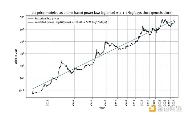
The model has attracted several critics, including Marcel Burger, Tim Stolte and Nick Emblow, who have each written "rebuttals" to the model. In this article, we aim to dissect one of the key arguments in these three criticisms: the alleged lack of cointegration between time and price, which dismisses the model as “invalid” and merely indicating a spurious relationship.

Is this really the case?

In this article, we will examine this issue thoroughly. This leads us to the conclusion that, strictly speaking, cointegration cannot exist in time-dependent models, including our own. Nonetheless, it is undeniable that one of the statistical properties necessary for cointegration exists in time-based power law models. Therefore, we conclude that time-based power laws are cointegrated in a loose sense, that our critics are wrong, and that the model is perfectly valid. We show that this conclusion holds equally well for the stock-to-flow (S2F) model and the exponential growth observed in long-term stock market index prices.

Introduction to concepts

Cointegration wtf

Are you already lost? Maybe the word "cointegration" is unfamiliar to you? Don’t worry: Judea Pearl, an expert in causal reasoning and non-spurious relationships and author of The Book of Why, claims to know nothing about the subject. We will endeavor to fully clarify the relevant terminology of the issue at hand.

Interesting and fascinating is the raging cointegration debate over X in the #bitcoin space, characterized by the apparent superficiality of the subject. Many followers of stock-flow and power laws are confused. Interested readers can see this for themselves by entering the search phrase "What is cointegration" into X. While some contributors appear to have mastered and refined their understanding over time, others remain confused, switch sides, or become disoriented. We have never discussed this topic until now.

First some background

Stochastic processes involve random variables. The value of a random variable is not predetermined. In contrast, a deterministic process can be predicted accurately in advance—every aspect of it is known in advance. Things like stock market prices are random because we cannot predict the price of an asset ahead of time. Therefore, we treat time series such as stock or Bitcoin prices as observations of random variables.

Instead, the passage of time follows a deterministic pattern. Every second, every passing moment passes - without any uncertainty. Therefore, the duration that elapses after an event occurs is a deterministic variable.

Stationality of a signal

Before studying cointegration, let us first take a look at the cointegration Basic concept of integration: stationarity:

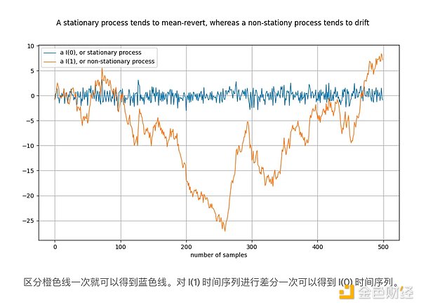
A stationary process is a stochastic process that, broadly speaking, has the same properties over time. Examples of such properties are the mean and variance, which are defined and stable for a stationary process. A synonym for stationary time series is I(0). Time series from stationary processes should not "drift" and should tend to return to the mean, usually zero.

An example of a non-stationary process is a random walk, which describes Brownian motion or particle diffusion in physics: each new value in a random walk depends Adds a random number to the previous value. The properties of a non-stationary process, such as mean and variance, vary over time or are not defined. Non-stationary processes are I(1) or higher, but usually I(1). Time series originating from non-stationary processes "drift" over time, that is, tend to move away from any fixed value.

The notation I(1) refers to the frequency at which the time series needs to be "differenced" before reaching stationary. Difference is the difference between a value in a time series and its previous value. This is roughly equivalent to taking the derivative. A stationary time series is already stationary - it needs to differ 0 times to be stationary, so it is I(0). The I(1) time series needs to be differentiated once before it becomes stationary.

The above figure is constructed by performing a difference on the orange time series to obtain the blue time series. Equivalently, the orange time series is obtained by integrating the blue time series.

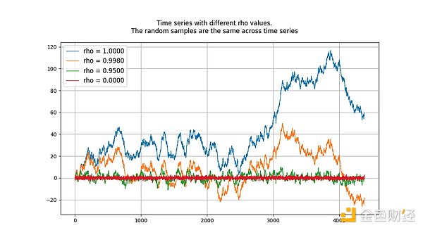
The unit root process here refers to an autoregressive model (more precisely of the AR(1) type) in which the rho parameter is estimated to be equal to 1. Although we use rho and root interchangeably, rho refers to processes that are often unknown and need to be estimated. The estimated result is the "root" value.

The value of rho represents the extent to which a process remembers its previous values. The value of u refers to the error term, assumed to be white noise.

The unit root process is a random walk and is non-stationary. Processes with "root" or rho values ​​below 1 tend not to drift and are therefore stationary. In the long run, even values ​​close to (but below) 1 will tend towards mean reversion (rather than drift). Therefore, a unit root process is special because it behaves fundamentally differently from processes whose roots are very close to 1. The figure below shows 4 samples of data generated by 4 known autoregressive processes, each with a different rho value.

Cointegration of two signals

Two random variables (in our case time The presence or absence of cointegration between sequences). In order for the pair to be cointegrated, both must be integrated in the same order and be non-stationary. Furthermore (and this is the key part), there must exist a stationary linear combination of the two time series.

Example of no cointegration signal

If the two time series are non-stationary, then Linear combinations (in which case we simply choose the difference between two time series) are often non-stationary as well:

Example of cointegrated signal

h2>

If two non-stationary time series drift "in the same way" over the long term, then a linear combination (here we choose r2–0.5*r1) can be stationary:< /p>

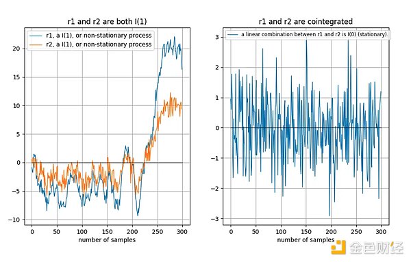
Tu et al. [1] provide a good visual description of cointegration:

"The existence of a cointegration relationship between time series means that they have a common random drift in the long run."

Why is it useful if two non-stationary time series have a stationary linear combination? Suppose we have two time series x and y, and we try to model y based on x: y = a + b*x. Our model error is given by the linear combination of x and y: model error = y — a — b*x . We hope that this model error is stable, that is, it does not drift in the long run. If model error peters out over the long term, that means our model is bad—incapable of making accurate predictions.

The devil is in the details

A more formal definition can be found in Engle and Granger's "Cointegration" and Error Correction: Representation, Estimation and Testing" [2] (Granger was the inventor of the concept of cointegration and received the 2003 Nobel Prize in Economics), which defines key concepts and tests for cointegration detection . The key to the paper is the assumption that the time series is stochastic and has no deterministic component (we will discuss this later).

Applied to time and Bitcoin price

In the case of a time-based power law, we There are two variables:

1. log_time: the logarithm of the number of days since the genesis block

2. log_price : logarithm of price

According to the definitions of Engle and Granger, both variables need to be random variables, have no deterministic components, and need to be non-stationary. Furthermore, we must be able to find a stationary linear combination of two variables. Otherwise, there is no cointegration between the two variables.

Before going into the details, let's first show some graphs on the model data itself, without any notion of stationarity or cointegration concepts. Note that the time-based power law produces a fit that looks pretty good visually. The residual vector does not immediately indicate drift.

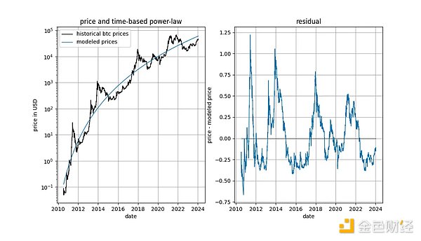
Furthermore, the model shows excellent out-of-sample performance (see below). Excellent out-of-sample performance is not consistent with the claim that the model is spurious - a model based on spurious correlations should be: spurious, meaning it cannot predict accurately. Out-of-sample performance can be tested by fitting the model to a limited amount of data (up to a certain date) and predicting the time period when the model does not fit (similar to cross-validation). During the out-of-sample period, observed prices continue to cross modeled prices frequently, and the largest excursions in observed prices do not move systematically away from modeled prices.

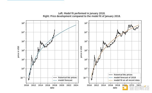
We can look more rigorously at the performance of the model after its release (September 2019) because we cannot cheat in any way after the model is released - we cannot change it after the fact Model.

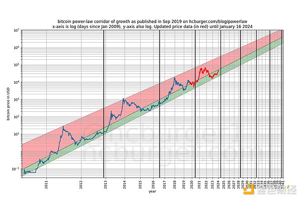
Any accusation that the model is based solely on spurious correlations should be taken with a grain of salt regarding the model's predictive power.

Cointegration step by step

In order to make it possible for cointegration between log_time and log_price, the two Each variable must be a random variable integral of the same order, and must be at least order 1.

log_price variable

Is log_price a stationary time series? Nick concludes that using the unspecified style ADF test (non-stationarity test) and the KPSS test (stationarity test), log(price) is undoubtedly non-stationary and therefore I(1) or higher. Marcel Burger concluded by visual inspection that I(1). Tim Stolte made a more interesting observation: he ran ADF tests on different time periods (no style specified) and noted that the situation is not clear-cut: "Therefore, we cannot firmly reject non-stationarity and conclude that there is a logarithmic price Signs of non-stationarity."

Let's conduct our own analysis. Similar to Tim Stolte, we will apply the ADF test at different time windows: always starting from the first available date and adding one day each day (we use daily data). This way we can see how the results of the ADF test change over time. But unlike Tim and Nick, we will specify which version of the ADF test to run. According to Wikipedia, DF and ADF tests come in three main flavors:

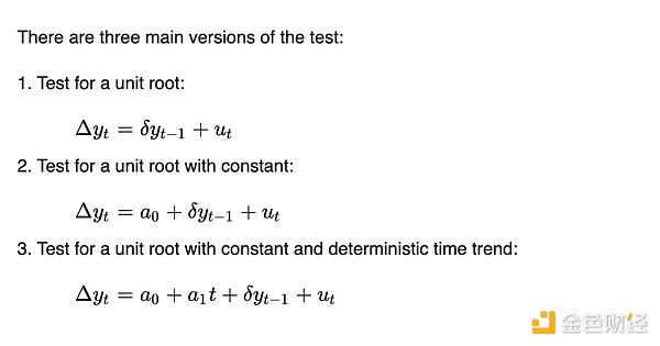
The difference between these three versions is their ability to accommodate (eliminate) different trends. This is related to Engle and Granger's requirement to remove any deterministic trends - these three versions are able to remove three simple deterministic trend types. The first version attempts to describe daily log_price changes using only past log_price data. The second version allows the use of a constant term, with the effect that log_price can have a linear trend (either upward or downward). The third version allows quadratic (parabolic) components.

We don't know which versions Tim and Nick are running, but we'll be running all three.

The maximum lag we used in our ADF tests was 1, but using longer lags did not significantly change our results and conclusions. We will use python's statsmodels.tsa.stattools.adfuller function, where "maxlag" is 1, and will use "n", "c" and "ct" as "regression" parameters (equivalent to the three described by Wikipedia above style) ). In the figure below, we show the p-value (a measure of statistical significance) returned by the test, where lower values ​​mean a higher likelihood of stationarity (usually a threshold of 0.05 is used).

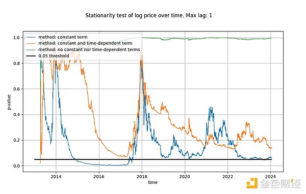
We observe that the first style (green line) clearly concludes that the log_price time series is non-stationary. A third version of the test (orange line) leads to the same conclusion, but is less decisive. Interestingly, a test that considers a constant term (blue line) cannot determine whether the time series is stationary (Tim most likely also used an ADF test with a constant term). Why are these three versions so different, and in particular why does the version with a constant term not exclude log_price from being stationary?

There can be only one explanation: using only a constant term in the log_price difference (resulting in a linear term in log_price) fits the time series "well", This results in a residual signal that appears almost stationary (albeit with considerable start and end deviations). So far, not using a deterministic trend at all in log_price, or using a quadratic deterministic effect, has worked poorly.

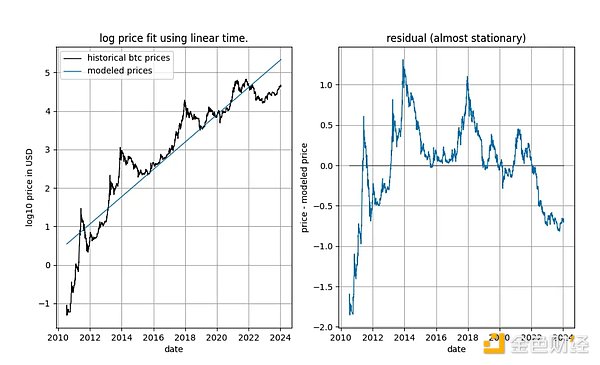
This already gives us a strong hint that there is a relationship between time and log_price. In fact, if an ADF test using a constant term concludes that the signal is stationary, this would mean that the linear time term is able to approximate log_price well enough to obtain a stationary residual. Obtaining stationary residuals is desirable because it is a sign of a non-spurious relationship (i.e. we have found the correct explanatory variables). A linear time trend isn't quite what we need, but it looks like we're pretty close.

Our conclusions differ significantly from those of Marcel Berg, who stated (in another article):

"In a previous analysis, I showed that the price of Bitcoin was integral to the first order, and it still is. Bitcoin is The evolution of prices over time does not exhibit any deterministic elements."

We conclude that linear time does not fully explain Bitcoin’s price action over time, but it is absolutely clear that log_price has a deterministic time element. Furthermore, it is not clear whether log_price is I(1) after removing the appropriate deterministic components (as required by Engel and Granger). Instead, it appears to be trend-stationary, but the appropriate deterministic component still needs to be found.

If we are looking for cointegration, the fact that log_price is not I(1) is already a problem, because for two variables to be cointegrated, they must All are I(1) or higher.

log_time variable

Now let's look at the log_time variable. Marcel Burger concluded that log_time appears to be a sixth-order integral (he kept the difference until he encountered numerical problems). The way he expected a mathematical function like the logarithm to transform from a completely deterministic variable to a random variable was absurd.

Nick comes to the same conclusion for the log_time and log_price variables: it is undoubtedly non-stationary and therefore I(1) or higher. Tim Stolte claims that log_time is non-stationary by construction. These are surprising statements! Integral order and cointegration refer to the concept of random variables and remove any deterministic trends from them (see Engle and Granger [2] above). As a reminder: the values ​​of deterministic variables are known in advance, whereas the values ​​of random variables are not. Time is (obviously) completely deterministic, and so is the logarithmic function, so log_time is also completely deterministic.

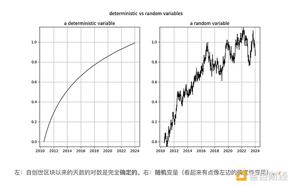
If we follow Engle and Granger and remove the deterministic trend from log_time, we are left with a vector of zeros because log(x) — log( x) = 0, i.e. we still have a completely deterministic signal. This means that we are stuck - we cannot transform the completely deterministic variable log_time into a random variable, so we cannot use Engle and Granger's framework.

Another way to understand how problematic a completely deterministic variable is in cointegration analysis is to consider how stationarity tests (such as the Dickey-Fuller test) Deal with it. Let us consider the simplest case (where y is the variable of interest, rho is the coefficient to be estimated, and u is the error term assumed to be white noise):

Should what happened? The error term u_{t} is 0 for all values ​​of t because we have no random components — no error is needed. But since log_time is a nonlinear function of time, the value of rho must also depend on time.

For random variables, this model is more useful because the variable rho captures the degree of memory of previous random values. But without random values, the model is meaningless.

Other types of tests suffer from the same problems as deterministic variables.

Therefore, completely deterministic variables do not belong to cointegration analysis. Or in other words: cointegration analysis does not work with deterministic signals, and if one of the signals is deterministic, cointegration analysis is an anachronistic tool for claiming spurious relationships.

What should I do?

Cointegration is defined only between two variables that are both I(d), where d is at least equal to 1. We have shown that log_time is a completely deterministic variable and cannot be used in stationarity tests. We cannot say whether log_time is I(0), I(1) or I(6). In addition, log_price is not I(1), but has a stationary trend.

Does the fact that there is no defined cointegration between log_time and log_price mean that time-based power laws are statistically invalid or spurious?

It is perfectly valid to use a mixture of deterministic and trend-stationary variables in any appropriate statistical analysis. As our critics would like to believe, cointegration is not the central point in the analysis of statistical relationships.

So cointegration is impossible. But stationarity analysis may still have a place when applied to power law models. Let’s explore this further.

The reason why we first conduct cointegration analysis between the input variables is because we hope to find a stationary linear combination of the two. There is no fundamental reason why it is not possible to combine a deterministic variable (log_time) and a trend-stationary variable (log_price) to obtain a stationary variable. Therefore, instead of looking for cointegration in the strict sense (since the residual is just a linear combination of the two input signals), we can simply perform a stationarity test on the residuals. If the residuals are stationary, we will find stationary linear combinations (which is the goal of cointegration) even if we do not strictly follow the Engel-Granger cointegration test.

Deeper Study

James G. MacKinnon in his paper "Cointegration Test This is explained accurately in "Critical value of "[3]: The cointegration test (Engle Granger test) is the same as the stationarity test of the residuals (DF or ADF test). If the "cointegration" regression" (replace log_time Regression linked to log_price) has been performed:

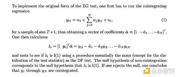
MacKinnon repeated this statement: If the parameters connecting log_time and log_price are known a priori, you can skip the Engle Granger cointegration test, and instead perform one of three common styles of stationarity tests (DF or ADF tests) on the residuals:

Therefore, we can use either of the two methods, which are identical except for the generated test statistic:

1. Fit log_time to log_price and calculate the residual (error). Based on this residual, calculate the DF or better ADF test. The resulting statistic tells us whether the residual Stationary.

2. Assume log_time and log_price are I(1), and run the Engle-Granger cointegration test. The resulting statistics also tell us whether the residuals are stationary.

For ADF test, use python’s statsmodels.tsa.stattools.adfuller function; for Engle-Granger test, we use statsmodels .tsa.stattools.coint. For both functions, we use the flavor that does not use constants (no constant drift over time) because our residuals should not contain constant drift over time (as that would mean Over time, the model begins to over- or under-price).

We wrote that the ADF and Engle-Granger tests are equivalent, but this is not entirely true: they do not produce the same test statistics. The Engle-Granger cointegration test assumes N=2 random variables, while the ADF test assumes N=1 random variable (N is a measure of degrees of freedom). A random variable can be affected by another random variable or a deterministic variable, but a deterministic variable cannot be affected by a random variable. Therefore, in our case (with only one deterministic variable log_time), the statistics returned by the ADF test (assuming N=1 random variables) are preferred. In principle, the Engle-Granger and ADF tests may be inconsistent, but in practice, this is not the case for time-based models. As shown in the figure below, the conclusion is the same: we get a stationary residual vector.

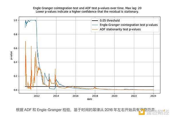
Neither test initially indicates stationary residuals, which is normal. This is because there are low-frequency components in the residual signal, which may be mistaken for non-stationary signals. Only over time does the residual mean recover significantly and become effectively stationary.

S2F and long-term stock index prices

The S2F model seems to have been generally ignored because strictly Cointegration on turns out to be impossible for a reason similar to that of time-based power laws: (partially) deterministic input variables. However, the residuals produced by the model appear to be very stable.

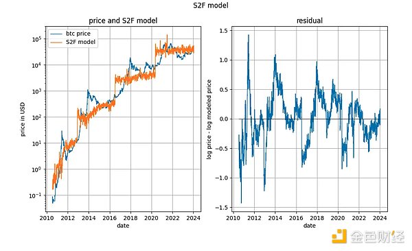
In fact, both the Engle-Granger cointegration test and the ADF stationarity test (preferred since there is a deterministic variable and a random variable) yield p very close to 0 value. Therefore, the basis for the S2F model's "lack of cointegration" (which actually means "lack of stationarity") should not be ruled out.

However, we pointed out in early 2020 that there are other signs that the S2F model should not hold. We predicted that BTCUSD price would be lower than the S2F model predicted, and this prediction proved to be prescient.

It's also interesting to look at long-term stock price indices versus time (here is the S&P 500 without reinvested dividends). It is known that major stock market indexes grow at an average index rate of around 7%. In fact, we confirm this with exponential regression.

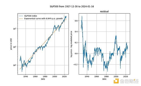
Here again we have a deterministic variable (time). The Engle Granger cointegration test yields a p-value of approximately 0.025, and the ADF test (preferred) yields a p-value of approximately 0.0075 (but these values ​​are highly dependent on the exact time period chosen). Again, the stationary residuals. Exponential time trends in stock prices are valid.

Impact

The S2F model was originally developed for its good econometric foundation (especially the association (especially Marcel Burger and Nick Emblow). As the tide turned and it was discovered that the S2F model could not exist for cointegration (in the strict sense), both Marcel and Nick jumped ship and declared the S2F model invalid. It seems that after this incident, people's views on the S2F model have also changed. Eric Wall has a great short summary of the turn of events.

We have explained, and the econometric literature (MacKinnon [3]) agrees with us, that cointegration and stationarity are almost interchangeable Use (except statistical values). Using this insight, we find that the S2F model does not have any problems with cointegration/stationarity, so it would be a mistake to change one's mind about the S2F model because of the assumed lack of cointegration. We agree that the S2F model is wrong, but it is wrong for reasons other than lack of cointegration.

Bitcoin's time-based power law has been criticized for its lack of cointegration, allegedly labeling the relationship between log_time and log_price as spurious. We have shown that Bitcoin’s time-based power law has apparently stationary residuals, so our critics’ line of reasoning makes no sense.

Bitcoin’s time-based power law model is effective, stable and powerful. as always.