Compiled by: Liu Jiaolian
Jiaolian Press:This article is translated from the paper "Bitcoin's Time Power Law Model and Its Analysis" by Harold Christopher Burger and Peter Vijn "Bitcoin's time-based power-law and cointegration revisited, 2024.1.31" is highly theoretical and suitable for readers with a certain statistical foundation. In order to facilitate the understanding of readers with insufficient basic knowledge, the teaching chain will first give some simple explanations.
As for the so-called time power law model, Jiao Lian has written many articles to introduce it in the past few years.
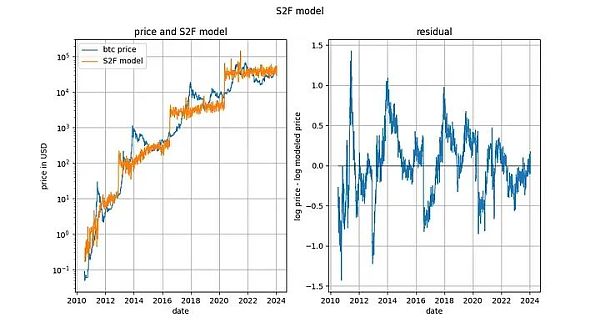
PlanB, a relatively well-known anonymous analyst in the industry, has always advocated using S2F hardness to model prices. This is the so-called S2F model. But alas: the S2F model is wrong. But please note that this does not mean that the S2F indicator is meaningless, it just means that the relationship between changes in S2F hardness and price is not as "radical" as PlanB depicts.
The following figure clearly shows the relative relationship between the power law model and the S2F model:

Obviously, the S2F model believes that the linear passage of time can drive the exponential growth of prices, while the power law model believes that the exponential passage of time can drive the exponential growth of prices.
The teaching chain prefers to use S2F hardness to visualize the "phase change" caused by the halving of output, but uses a power law model to transform Bitcoin into a log-log space for linear regression. The elegance of the power law model is particularly similar to the support vector machine (SVM), so it is very suitable for me.
The following is the paper by H. Burger & P. Vijn. Enjoy!
* * *
Introduction
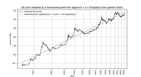
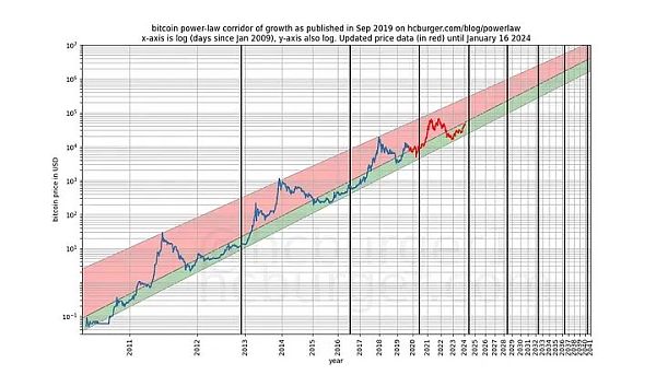
Bitcoin’s time-based power law, initially Proposed by Giovanni Santostasi in 2014 and reformulated by us in 2019 (as a corridor or three-parameter model), it describes the relationship between Bitcoin price and time. Specifically, the model describes the linear relationship between the logarithm of the number of days since Bitcoin’s genesis block and the logarithm of Bitcoin’s USD price.

The model attracted designers including Marcel Burger, Tim Stolte and Nick Emblow Several critics have written articles "refuting" the model. In this article, we will unpack one of the key arguments in each of these three criticisms: the claim that there is no cointegration between time and price, arguing that the model is "invalid" and simply indicates a spurious relationship.
Is this really the case?
In this article, we will take a closer look at this issue. This leads us to conclude that, strictly speaking, cointegration cannot exist in time-dependent models, including our own. However, it is undeniable that one of the statistical properties necessary for cointegration exists in time-based power law models. Therefore, we conclude that the time-based power law model is cointegrated in the narrow sense, that our criticism is misplaced, and that the model is perfectly valid. We show that this conclusion holds equally well for the Stock-to-Fund ratio (S2F) model and the exponential growth observed in long-term stock market index prices.
Introduction to concepts
What is cointegration
Have you lost your way? Maybe you're not familiar with the term "cointegration"? Don’t worry: Judea Pearl, an expert in causal inferences and non-spurious relationships and author of The Book of Why , claims to know nothing about the subject. We will endeavor to fully clarify the relevant terms at hand.
The debate over cointegration in Bitcoin-related discussions on Twitter is very interesting and quite fascinating. Many followers of stock-to-increase ratios and power laws are confused. Interested readers can see this for themselves by searching for “what is cointegration”. Over time, some contributors appear to have mastered and refined their understanding, while others remain confused, switch sides, or become disoriented. Only now are we paying attention to this topic.
Some background information first
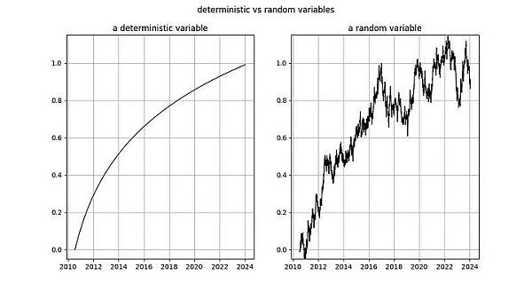
Stochastic processes involve random variables. The value of a random variable is not predetermined. In contrast, a deterministic process can be predicted accurately in advance – every aspect of it is known in advance. Stock market prices, etc. are random variables because we cannot predict the price of an asset in advance. Therefore, we treat time series such as stock or Bitcoin prices as observations of random variables.
Instead, the passage of time follows a deterministic pattern. Every second passes without any uncertainty. Therefore, the duration after an event occurs is a deterministic variable.
The stationarity of a signal
Before studying cointegration, let us first take a look at the basic concept of cointegration: stationary: < /p>

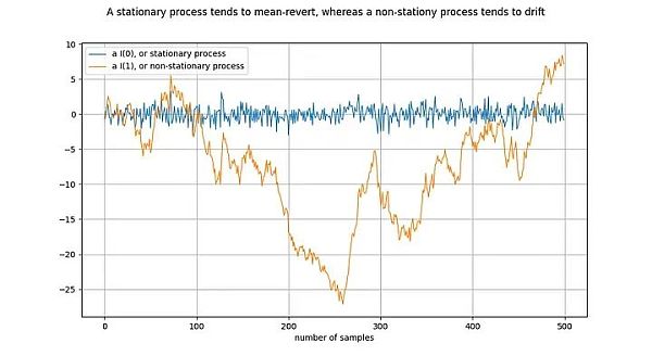
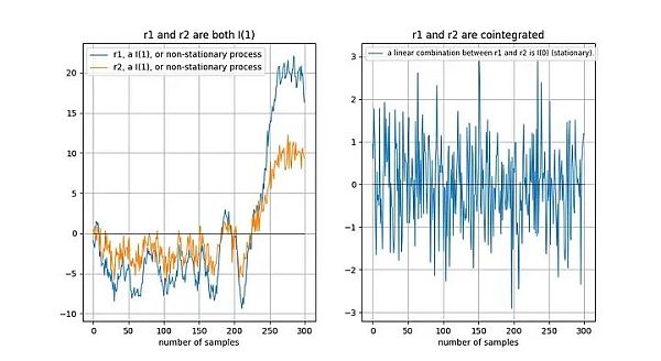
Illustration: Differentiate the orange line once to get the blue line. Difference the I(1) time series once to get the I(0) time series.
Stationary process (stationary process) is a stochastic process, broadly speaking, it has the same properties over a period of time. For example, for a stationary process, its mean and variance are determined and stable. A synonym for stationary time series is I(0). Time series derived from stationary processes should not "drift" but should tend to the mean value, usually zero.
An example of a non-stationary process is a random walk, such as Brownian motion or particle diffusion in physics: each new value in a random walk depends on the previous value plus a random number. The properties of a non-stationary process, such as mean and variance, change over time or are not defined. Non-stationary processes are I(1) or higher, but usually I(1). Time series originating from non-stationary processes will "drift" over time, i.e., tend to deviate from any fixed value.
The notation I(1) refers to how many times a time series needs to be "differenced" to reach stationarity. Difference means finding the difference between a value in a time series and its previous value. This is roughly equivalent to taking the derivative. A stationary time series is already stationary - it takes 0 differences to become stationary, so it is I(0). The I(1) time series needs to be differentiated once to reach stationary.
The above figure is drawn by performing a difference on the orange time series to obtain the blue time series. Equivalently, the orange time series is obtained by integrating the blue time series.
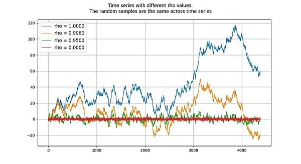
The unit root process refers to autoregressive models (more precisely of the AR(1) type) whose rho parameters are estimated is equal to 1. Although we can use rho and root interchangeably, rho refers to the true value of the process, which is usually unknown and needs to be estimated. The estimated result is the "root" value.
The value of rho indicates how well the process remembers previous values. The value of u refers to the error term, assumed to be white noise.

The unit root process is a random walk process and is a non-stationary process. Processes with "root" or rho values below 1 tend not to drift and are therefore stationary. Even values close to (but below) 1 tend to mean reversion (rather than drift) in the long run. The peculiarity of a unit root process is therefore that it is fundamentally different from processes whose roots are very close to 1.

Cointegration of two signals
The presence or absence of cointegration (cointegration relationship) between two random variables (in this case, time series). For this pair of variables to have a cointegrating relationship, both must have the same integration order and both must be non-stationary. Furthermore (and this is the key part), the linear combination of two time series must be stationary.
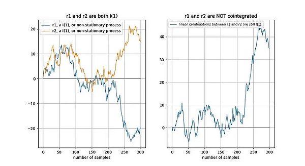
Example of signal without cointegration
If two time series are non-stationary, then a linear combination (in this case, we only need to choose two The difference between time series) is usually non-stationary:

Cointegration signal example
If two non-stationary time series drift "in the same way" in the long run, then a linear combination (here we choose r2-0.5*r1) is possible is stationary:

Tu et al. [1] intuitively described cointegration Relationship:
"The existence of a cointegration relationship between time series means that they have a common random drift in the long run".
Why is the linear combination of two non-stationary time series stationary? Suppose we have two time series x and y, and we try to model y based on x: y = a + b*x. Our model error is given by the linear combination of x and y: model error error = y - a - b*x . We want the model error to be stationary, that is, not drift over the long term. If the model error drifts over time, it means our model is not good and cannot make accurate predictions.
Details are the devil (details determine success or failure)
In Engle and Granger [2] (Granger is the invention of the concept of cointegration In his article "Cointegration and Error Correction: Representation, Estimation and Testing" (who won the 2003 Nobel Prize in Economics), he defined the key concepts and testing methods of cointegration. The key to the paper is the assumption that the time series is stochastic and has no deterministic component (we'll get to that later).

If a deterministic trend exists, it should be removed before analysis:< /p>

Applied to time and Bitcoin price
In a time-based power law, we have two variables:
1. log_time: the logarithm of the number of days since the genesis block
2. log_price: price The logarithm of
According to the definitions of Engle and Granger, both variables must be random variables, have no deterministic components, and must be non-stationary. Furthermore, we must be able to find a static linear combination of these two variables. Otherwise, there is no cointegration relationship between the two variables.
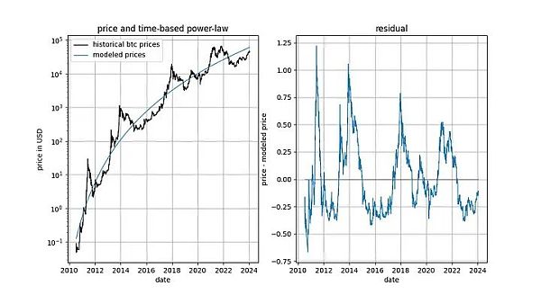
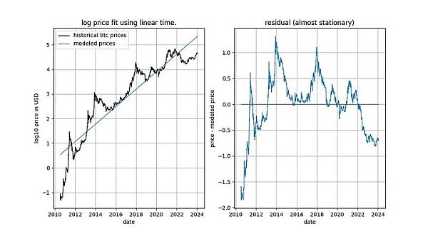
Before we dive into the details, let's show a few graphs of the model data itself, which does not include any notion of stationarity or cointegration. Note that the time-based power law produces a fit that seems intuitively good. The residuals vector does not immediately show drift.

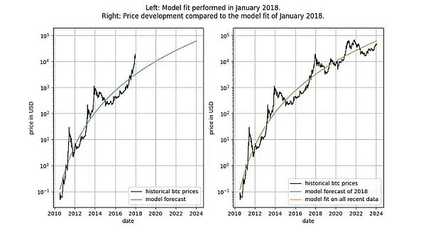
In addition, the model also shows excellent out-of-sample performance (see below) . Excellent out-of-sample performance does not mean that the model is spurious - a model based on spurious correlations should simply be spurious, i.e. fail to predict accurately. A way to examine out-of-sample performance is to fit the model on a limited amount of data (as of a certain date) and make predictions for the time periods when the model is not fitted (similar to cross-validation). During the out-of-sample period, observed prices frequently cross modeled prices, and the largest deviations of observed prices do not systematically move further away from modeled prices.

We can be more rigorous and observe the results after the model is released (September 2019) Performance, because after the model is released, we cannot cheat in any way - we cannot change the model after the fact.

If anyone accuses the model of being based only on a false correlation, then that The predictive power of the model should already be in doubt.
Gradually realize cointegration
To make it possible for a cointegration relationship to exist between log_time and log_price, the two variables must be random variables of the same order, and It is a random variable of at least order 1.
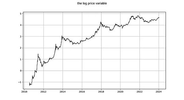
log_price variable

Is log_price a stationary time series? Nick uses the unspecified ADF test (non-stationarity test) and the KPSS test (stationarity test) to conclude that log(price) is undoubtedly non-stationary and therefore I(1) or higher. Marcel Burger concluded by visual inspection that it is I(1). Tim Stolte makes a more interesting observation: he performs an ADF test (unspecified type) for different periods and points out that the situation is not straightforward: "We cannot therefore firmly reject non-stationarity and conclude that there is a non-stationarity in log-price Conclusions for signs of stationarity."
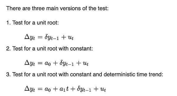
Let's run the analysis ourselves. Similar to Tim Stolte, we will perform the ADF test on different time windows: always starting from the first available date and increasing by one day each day (we use daily data). This way, we can see how the results of the ADF test change over time. But unlike Tim and Nick, we want to specify which version of the ADF test to run. According to Wikipedia, there are three main types of DF and ADF tests:

These three Versions differ in their ability to accommodate (remove) different trends. This is related to Engle and Granger's requirement to remove any deterministic trends - these three versions are able to remove three simple deterministic trend types. The first version attempts to describe daily log_price changes using only past log_price data. The second version allows the use of a constant term, with the effect that log_price can have a linear trend (either upward or downward). The third version allows quadratic (parabolic) components.
We don't know which version Tim and Nick are running, but we'll be running all three.
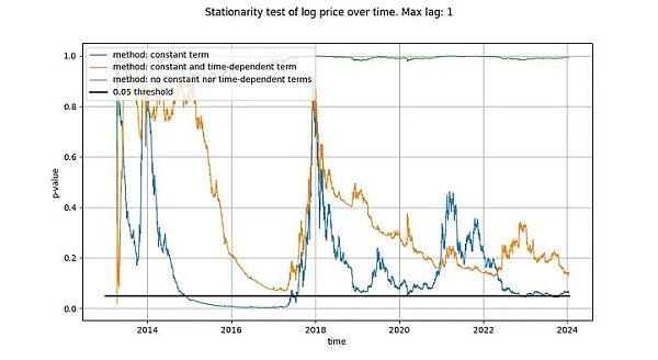
The maximum lag we use in our ADF tests is 1, but using longer lags does not meaningfully change our results and conclusions. We will use python's statsmodels.tsa.stattools.adfuller function with "maxlag" of 1 and "n", "c" and "ct" (equivalent to the three types described above in Wikipedia) for the "regression" parameter. In the image below, we show the p-value (a measure of statistical significance) returned by the test, with smaller p-values indicating a greater likelihood of stationarity (a commonly used critical value is 0.05).

We noticed that the conclusion drawn by the first method (green line) Yes, the log_price time series is non-stationary. The conclusion of the third test (orange line) is the same, but less decisive. Interestingly, the test that allows a constant term (blue line) cannot tell whether the time series is stationary (most likely Tim also used the ADF test with a constant term). Why are these three versions so different, and in particular why the version with a constant term cannot rule out that log_price is stationary?
There is only one explanation: using only a constant term in the log_price difference (resulting in a linear term in log_price) fits the time series "well", resulting in a residual signal that looks almost stationary (Although the deviation between the start and end points is quite large). Not using deterministic trends in log_price at all, or using quadratic term deterministic effects, are far less effective.

This has given us a strong hint that the relationship between time and log_price There is a relationship. In fact, if an ADF test using a constant term concludes that the signal is stationary, this means that the linear time term approximates log_price well, resulting in stationary residuals. Obtaining stationary residuals is desirable because it is a sign of a non-spurious relationship (i.e. we have found the correct explanatory variables). A linear time trend isn't quite what we want, but we seem to be getting close to it.
Our conclusions differ significantly from those of Marcel Burger, who (in another article) said:
“In a previous analysis, I showed that Bitcoin It remains valid that the price of is first-order integrated. Bitcoin does not exhibit any deterministic elements in its price evolution over time."
Our conclusion is that linear Time does not fully explain the behavior of Bitcoin's price over time, but it is absolutely clear that log_price has a definite time element. Furthermore, it is not clear whether log_price is I(1) after removing the appropriate deterministic components (as required by Engle and Granger). Instead, it appears to be trend-stationary, but an appropriate deterministic component still needs to be found.
If we are looking for a cointegration relationship, it is already a problem that log_price is not I(1), because for two variables to be cointegrated, they must both be I(1) or higher.
log_time variable

Now let's look at the log_time variable. Marcel Burger concluded that log_time seemed to be integrating to order 6 (he had been doing differentiation until he ran into numerical problems). His expectation that a mathematical function like the logarithm could be transformed from a completely deterministic variable into a random variable made no sense.
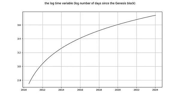
Nick's conclusion for log_time is the same as for the log_price variable: it is undoubtedly non-stationary and therefore I(1) or higher. Tim Stolte claims that log_time is non-stationary by construction. These statements are surprising! Integral order and cointegration refer to the concept of random variables in which any deterministic trend has been eliminated (see Engle and Granger [2] above). What needs to be reminded is that the value of a deterministic variable is known in advance, while the value of a random variable is unknown. Time is (obviously) completely deterministic, and so is the logarithmic function, so log_time is also completely deterministic.

Illustration: Left: The logarithm of the number of days since the genesis block is completely deterministic. Right: Random variable (looks a bit like the deterministic variable on the left).
If we follow Engle and Granger's method and remove the deterministic trend from log_time, then what remains is a zero vector, since log(x) - log(x) = 0 , that is, we still have a completely certain signal. This means we're stuck - we can't convert log_time, a completely deterministic variable, into a random variable, so we can't use Engle and Granger's framework.
Another way to see how problematic a fully deterministic variable would be in a cointegration analysis is to consider how a stationarity test such as the Dickey-Fuller test handles it. Let's consider the simplest case (where y is the variable of interest, rho is the coefficient to be estimated, and u is the error term assumed to be white noise):

What will happen? The error term u_{t} is 0 for all values of t because we have no random component - no error should be needed. But since log_time is a nonlinear function of time, the value of rho must also depend on time.
This model is more useful for random variables because the variable rho captures how well the previous random values have been remembered. But without random values, the model is meaningless.
For deterministic variables, other types of tests have the same problem.
Therefore, completely deterministic variables do not belong to the scope of cointegration analysis. Or to put it another way: cointegration analysis does not work with deterministic signals, and if one of the signals is deterministic, then cointegration analysis is an anachronistic tool that claims a spurious relationship.
How to explain
A cointegration relationship exists only when both variables are I(d) and d is at least equal to 1. We have shown that log_time is a completely deterministic variable and cannot be used for static testing. We cannot tell whether log_time is I(0), I(1), or I(6). In addition, log_price is not I(1), but has a stationary trend.
There is no cointegration relationship between log_time and log_price. Does this mean that time-based power laws are statistically invalid or spurious?
Of course not
In any appropriate statistical analysis, it is entirely correct to use mixed deterministic and trend-stationary variables of. Cointegration is not, as our critics would have you believe, a central point in the analysis of statistical relationships.
Therefore, cointegration analysis is not feasible. However, there may be a place for stationary analysis applied to power-law models. Let's explore this further.
The reason why we first conduct cointegration analysis on the input variables is because we hope to find a stationary linear combination of the two. It is fundamentally impossible to combine a deterministic variable (log_time) and a trend-stationary variable (log_price) to get a stationary variable. Therefore, instead of looking for a cointegration relationship in the strict sense, we can simply perform a stationarity test on the residuals (since the residuals are just a linear combination of the two input signals). If the residuals are stationary, then we find a stationary linear combination even though we do not strictly follow the Engle-Granger cointegration test (which is the purpose of cointegration).
In-depth discussion
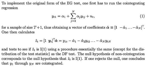
James G. MacKinnon [3] explains exactly this in his paper "Critical Values for Cointegration Tests": If A "cointegration regression" (a regression relating log_time to log_price) is performed, then the test for cointegration (Engle-Granger test) is the same thing as the test for stationarity of the residuals (DF or ADF test):

MacKinnon repeated this statement: If the parameters connecting log_time and log_price are a priori If you know, you can skip the Engle-Granger cointegration test and instead perform one of the three common types of stationarity tests (DF or ADF test) on the residuals:

Therefore, we can use either of the two methods, except for the resulting test statistic. are the same:
1. Fit log_time and log_price and calculate the residual (error). Calculate DF, or better yet ADF test, from the residuals. The resulting statistic tells whether the residuals are stationary.
2. Assume log_time and log_price are I(1) and run the Engel-Granger cointegration test. The resulting statistics can also indicate whether the residuals are stationary.
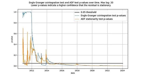
For the ADF test, we use python's statsmodels.tsa.stattools.adfuller function; for the Engle-Granger test, we use statsmodels.tsa.stattools.coint. For both functions, we used the method of not using a constant (not drifting over time) because our residuals should not contain drifting over time (because this means that over time, the model starts to overestimate or underestimate the price).
We wrote that the ADF test and the Engle-Granger test are equivalent, but this is not the case: they do not produce the same test statistics. The Engle-Granger cointegration test assumes N=2 random variables, while the ADF test assumes N=1 random variables (N is a measure of degrees of freedom). A random variable can be affected by another random variable or a deterministic variable, but a deterministic variable cannot be affected by a random variable. Therefore, in our case (with only one deterministic variable log_time), the statistic returned by the ADF test (assuming N=1 random variables) is preferable. In principle, the Engle-Granger test and the ADF test may diverge, but in time-based models, this is not the case in practice. As shown in the figure below, the conclusion is the same: we get a stationary residual vector. The scores for both tests are well below the 0.05 critical value (indicating that the residuals are stationary), and have remained so for a long time.

Illustration: The time-based power law has stationary residuals starting around 2016, according to the ADF and Engle-Granger tests.
Neither test initially showed that stationary residuals were normal. This is because the low-frequency components in the residual signal can be mistaken for non-stationary signals. Only over time does the mean reversion of the residuals become apparent and, in effect, stationary.
S2F and long-term stock index prices
The S2F model is generally rejected, seemingly because cointegration in the strict sense has been proven to be impossible. Similar to a time-based power law: the input variables are (partially) deterministic. However, the model produces residuals that appear to be very stationary.

In fact, the Engle-Granger cointegration test and the ADF stationarity test (because There is a deterministic variable and a random variable, so it is more preferable) and the resulting p-values are all very close to 0. Therefore, S2F models should not be excluded on the grounds of "lack of cointegration" (actually "lack of stationarity").
However, we noted in early 2020 that there were other signs that the S2F model did not hold. Our prediction that the price of BTCUSD would be lower than predicted by the S2F model proved to be prescient.
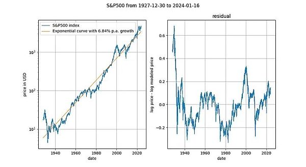
It is also interesting to look at long-term stock price indexes versus time (here the S&P 500 without dividend reinvestment). It's no secret that major stock market indexes grow at an average exponential rate of around 7%. In fact, we also confirmed this through exponential regression.

Here, we encounter another deterministic variable (time). The Engle-Granger cointegration test gives a p-value of about 0.025, and the ADF test (preferred) gives a p-value of about 0.0075 (but these values depend heavily on the exact time period chosen). Again, stationary residuals. Exponential time trends in stock prices are valid.
Impact
The S2F model was initially highly regarded (particularly by Marcel Burger and Nick Emblow) due to its purportedly good econometrics basis, especially the existence of cointegration relationships. As the tide turned, it became clear that the S2F model was not strictly cointegrated, and both Marcel and Nick jumped ship, declaring the S2F model invalid. It seems that public opinion of the S2F model also changed after this incident. Eric Wall has an excellent short summary of the turn of events.
We have explained, and the econometric literature (MacKinnon [3]) agrees with us, that cointegration and stationarity can be used almost interchangeably (except for the value of the statistic). According to this view, we do not believe that the S2F model has any problems with cointegration/stationarity, and therefore it would be a mistake to change one's view on the S2F model because of the alleged lack of cointegration. We agree that the S2F model is wrong, but the reason for its wrongness is not a lack of cointegration.
Bitcoin’s time power law model has been criticized for its lack of cointegration, which is said to signal that the relationship between log_time and log_price is spurious. We have shown that the residuals of Bitcoin's time-based power law model are clearly stationary, so the critics' reasoning is questionable.
Bitcoin’s time power law model is effective, stable and powerful. as always.
References
1. "Universal Cointegration and Its Applications" Tu et al., including supplemental information
2. “Co-Integration and Error Correction: Representation, Estimation, and Testing” by Robert F. Engle and C. W. J. Granger
3. "Critical Values for Cointegration Tests", James G. MacKinnon
 Joy
Joy


